

Welcome!
In this first tutorial, we'll see how to transform a disorganized, unusable Excel file into a beautiful SharePoint list!
Prerequisites for the tutorial :
Excel
SharePoint
I strongly encourage you to do the exercise, following the explanations as you go along.
You can download the Excel file I used as an example below:
This is the basis of our work.
The format of this "table" is not correct: the data is not organized in columns, there are typing errors...
Let me tell you this straight : As it stands, we can't do anything with this Excel file.
We absolutely must transform it before we can convert it into a SharePoint list.
The first thing is to determine the names of the columns we're going to create.
For example, we want :
Date
Order number
Destination
Carrier
An optional comment on the nature of the package (dangerous, fragile, etc.)
Order status
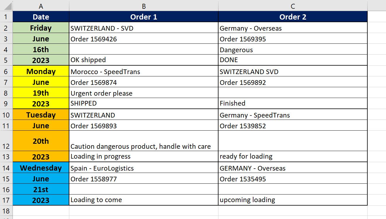
So we'll write the names of these 6 columns next to our good old table like this:
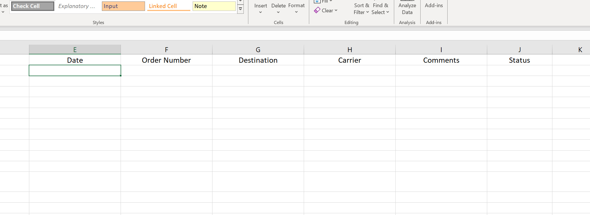
Once this has been done, we need to create a Table.
To do this, we'll select our cells as follows:
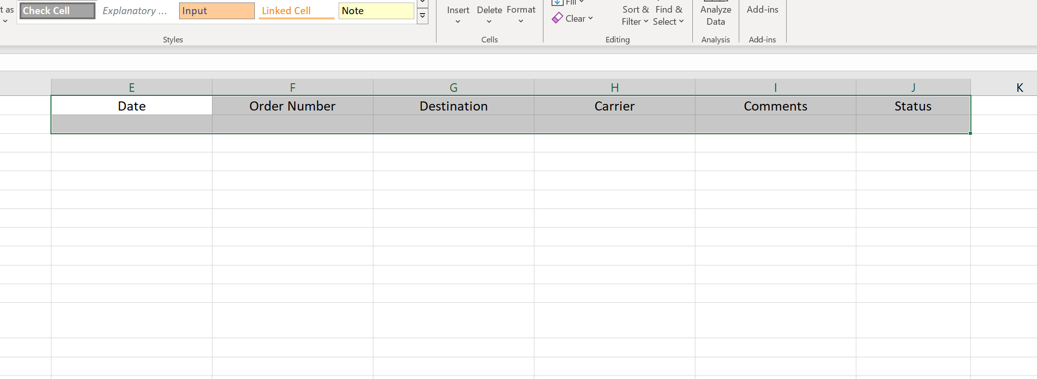
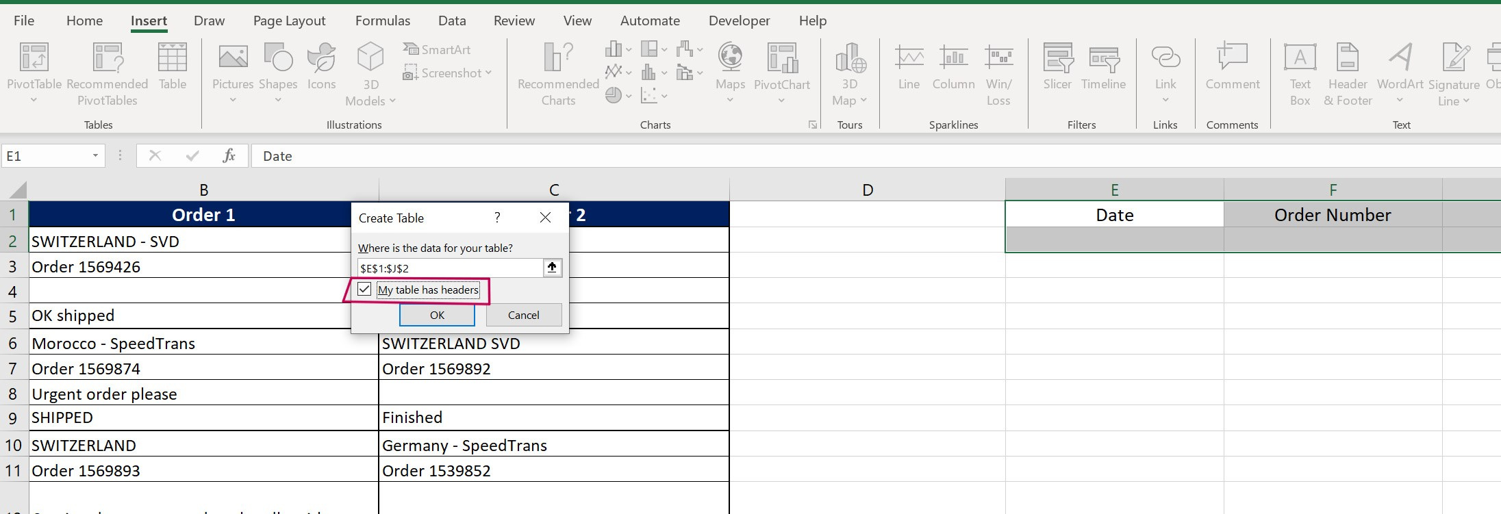
Next, we'll go to Insert and click on Table :
In the small window that opens, we select "My table has headers" :
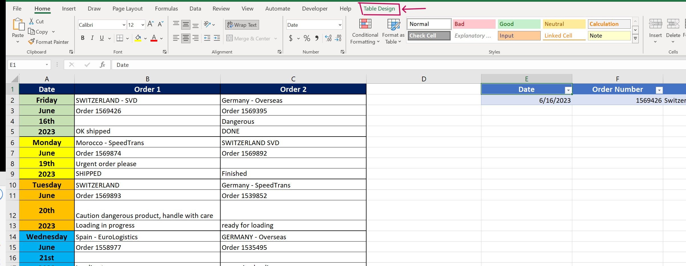
You can now see that our cells have changed color and that Excel considers this to be a Table, thanks to the appearance of "Table Design" in the Ribbon.
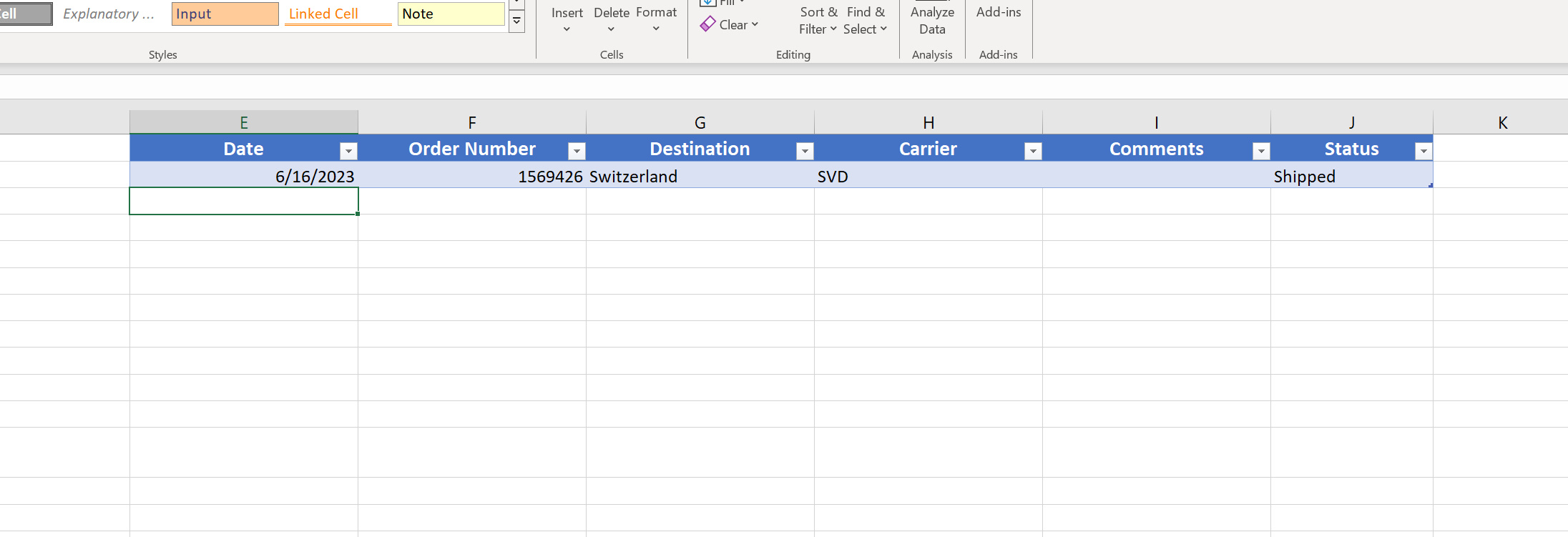
Now we'll need to add the data from our original table to the new one, respecting the corresponding columns.
For the first command in our previous table, here's what it should look like in the new one:
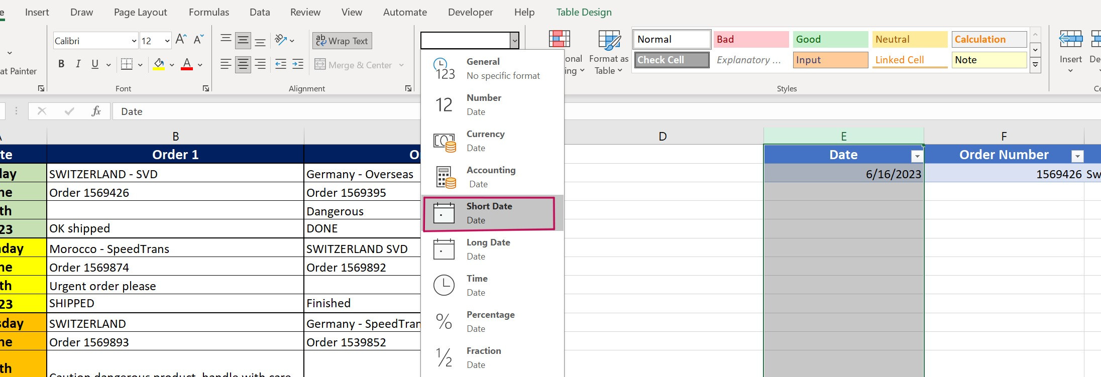
Important action:
Select column E, click on Home in the ribbon.
Change the format by clicking on "Short Date" as shown below.
This will be mandatory later on:
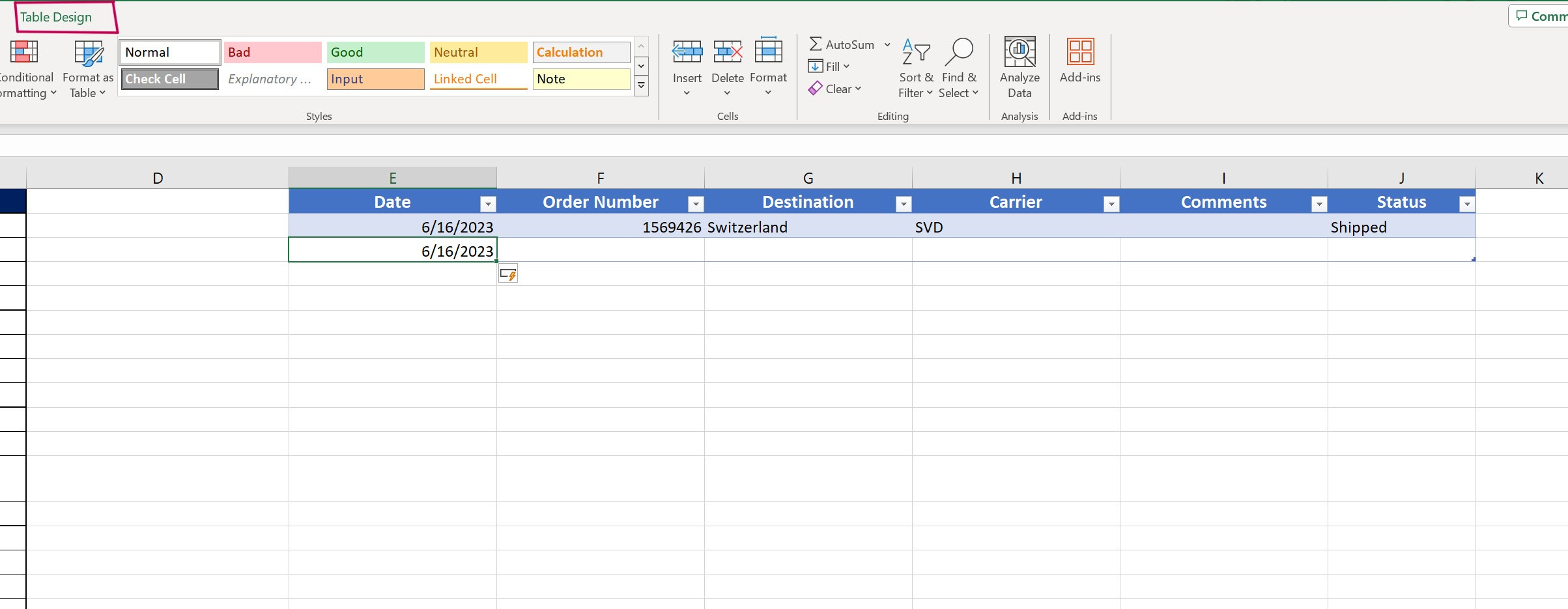
We can now move on to the second record.
Simply click on cell E3 and add the date of the second order. A new line should have been created automatically (you can see this by the blue border around the line and the presence of "Table Design" in the Ribbon).
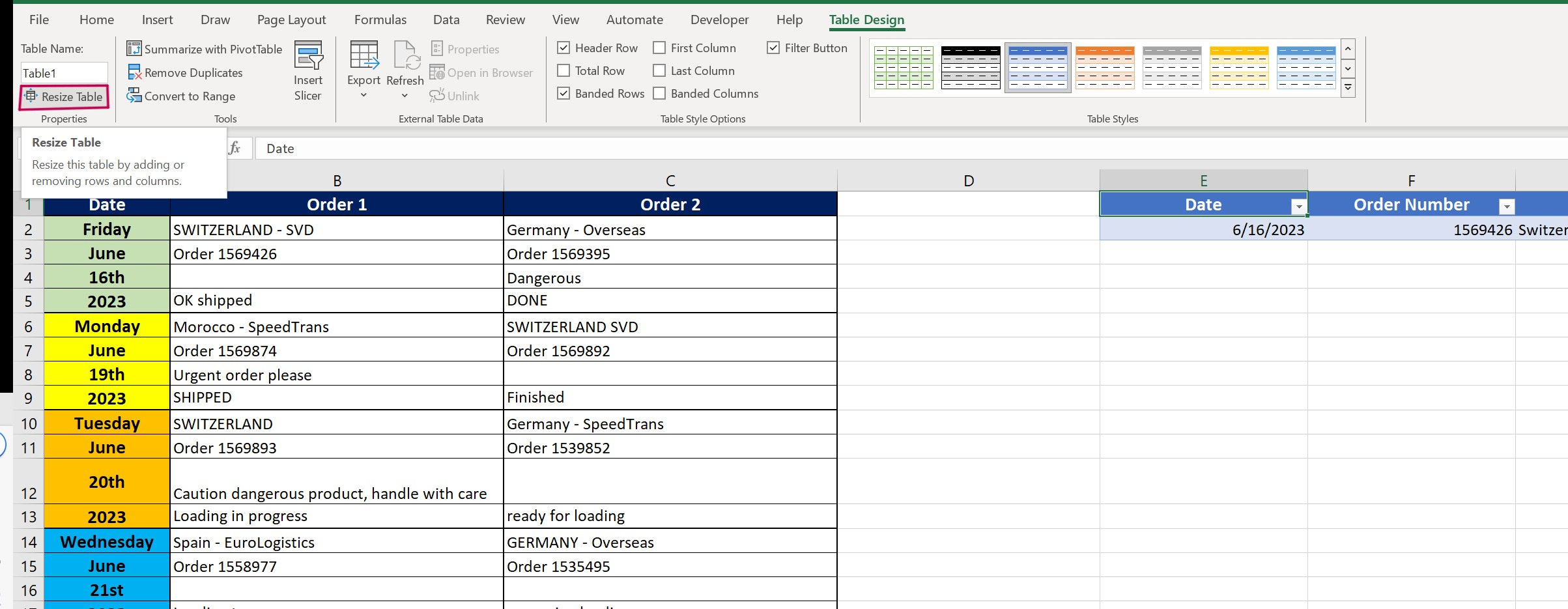
If not: click on cell E1 ("Date") and go to "Table Design" (as indicated in my screenshot):
Then go to "Resize Table" :
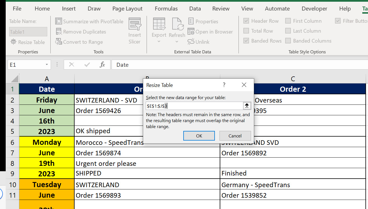
Then widen the scope of the Table by renaming "$E$1:$J$2" to "$E$1:$J$3" and click Ok.
Once you've added the new line, continue in the same way until you're satisfied with the data you've added.
Best practice: Have only one way of saying that the order has been dispatched. The same applies if the order is in progress or still to come.
For example, write only: Shipped, In progress or Upcoming, as shown below.
We'll see why a little later.
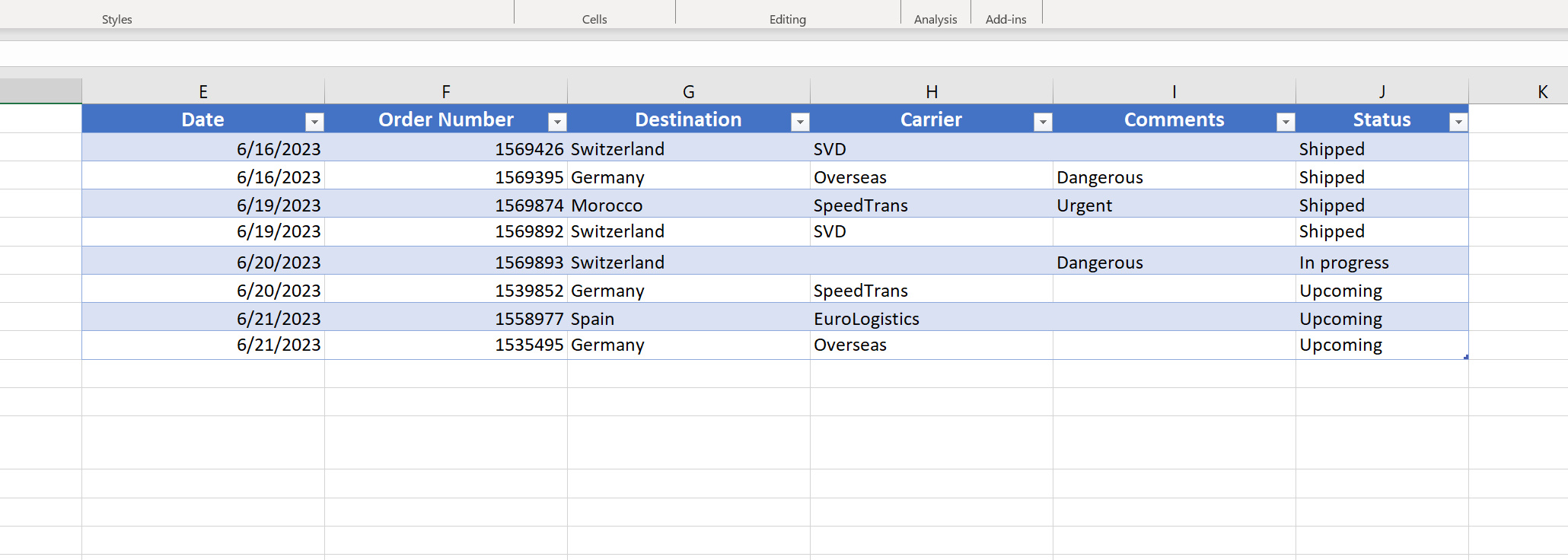
The final table should look like this:
Now it's time to convert our Table into a Sharepoint list!
First of all, save your file in your Documents, for example.
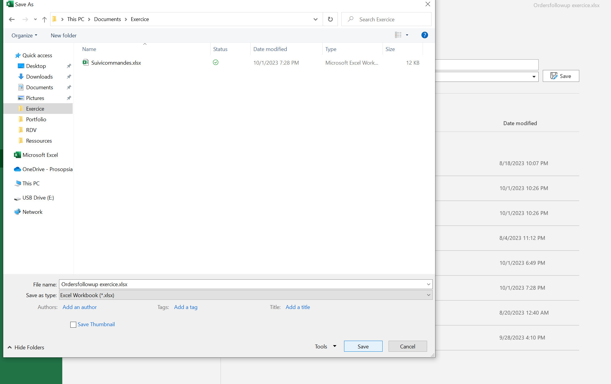
You can close the Excel workbook; we don't need it anymore.
We'll now go to our SharePoint site to create the new list.
(I take this opportunity to tell you that we'll be customizing our SharePoint site in a future post).
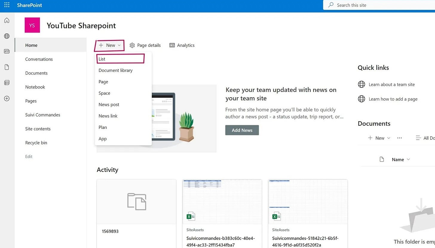
Click on the "+ New" button and select "List":
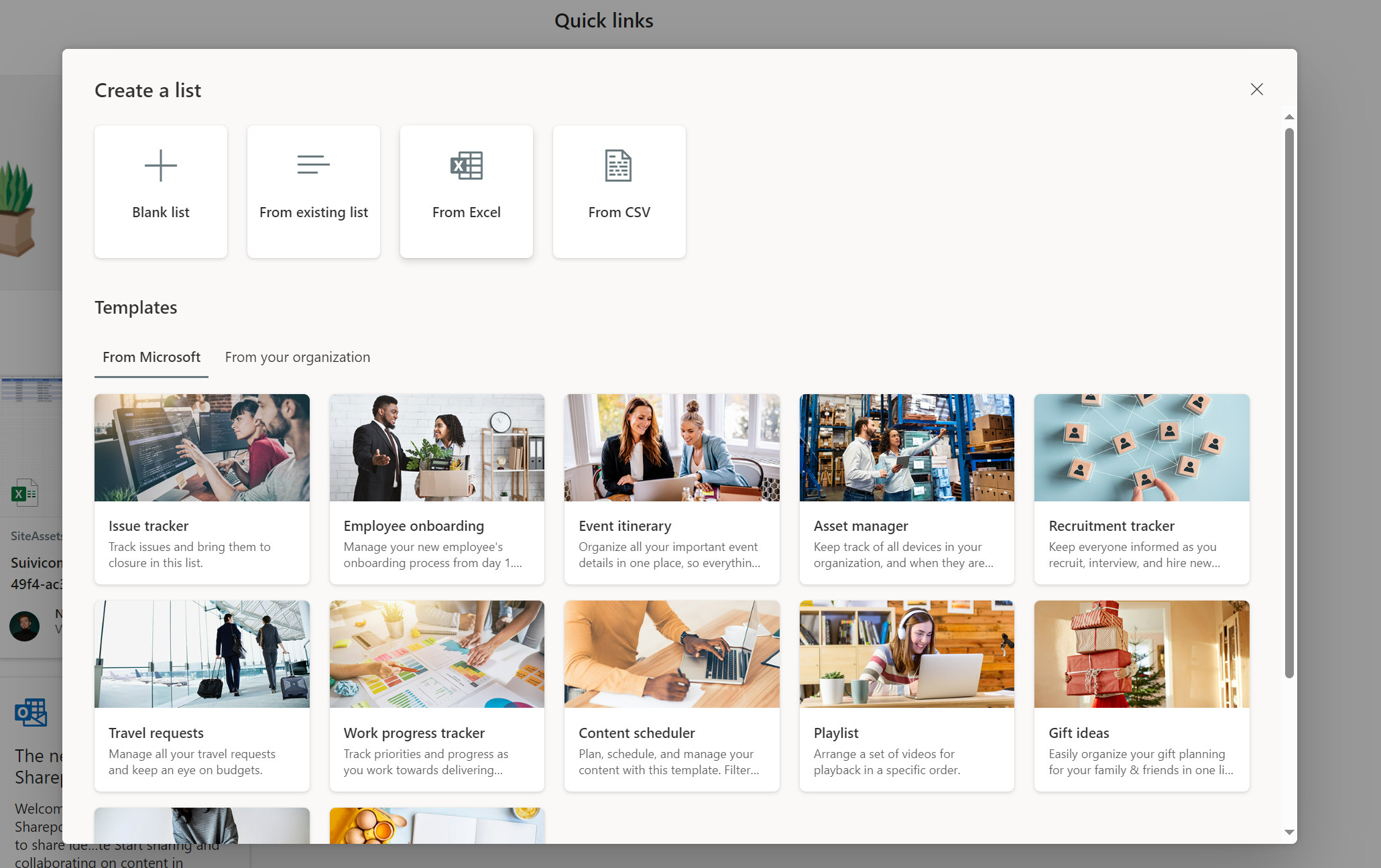
A window appears in which we simply select: "From Excel".
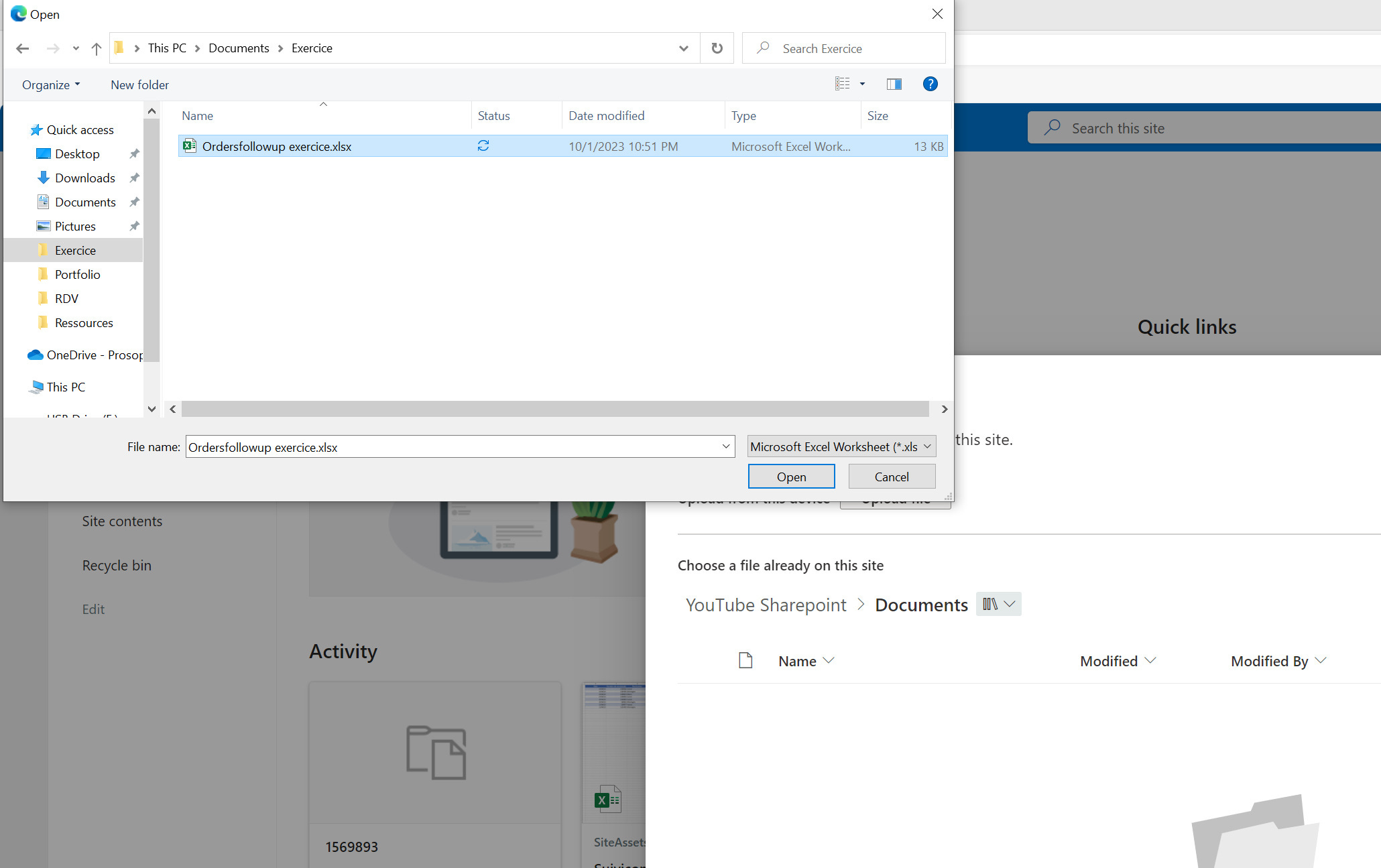
Click on "Upload file" to retrieve the Excel file we saved earlier (if you can't open it, you haven't closed the Excel file).
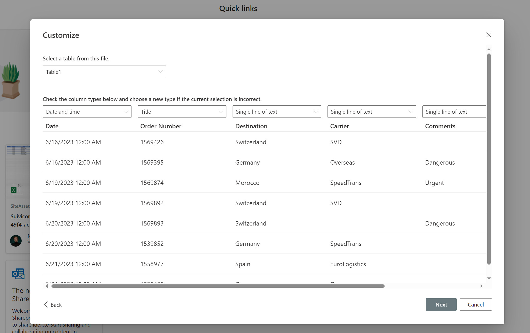
We're near the end! Now we need to tell which categories we want to assign to our columns.
Notice something interesting: it only suggests "Table1", as the previous table with our bulk data is not recognized by SharePoint.
The whole point of building an Excel Table as we've just done is that it becomes usable when we want to perform this kind of operation.
Remember:
If you need to create a new Excel workbook with data = create a table with the format I showed you earlier.
I recommend assigning the "Title" type to the "Order number" column. This is because order numbers are unique, unlike dates. On the other hand, this is the most important piece of information in our records. The destination, status, etc. are only information that serves the order number.
We therefore change the "Number" category automatically assigned by SharePoint to the "Title" category, and take advantage of this to assign the "Date and time" category to our "Date" column:
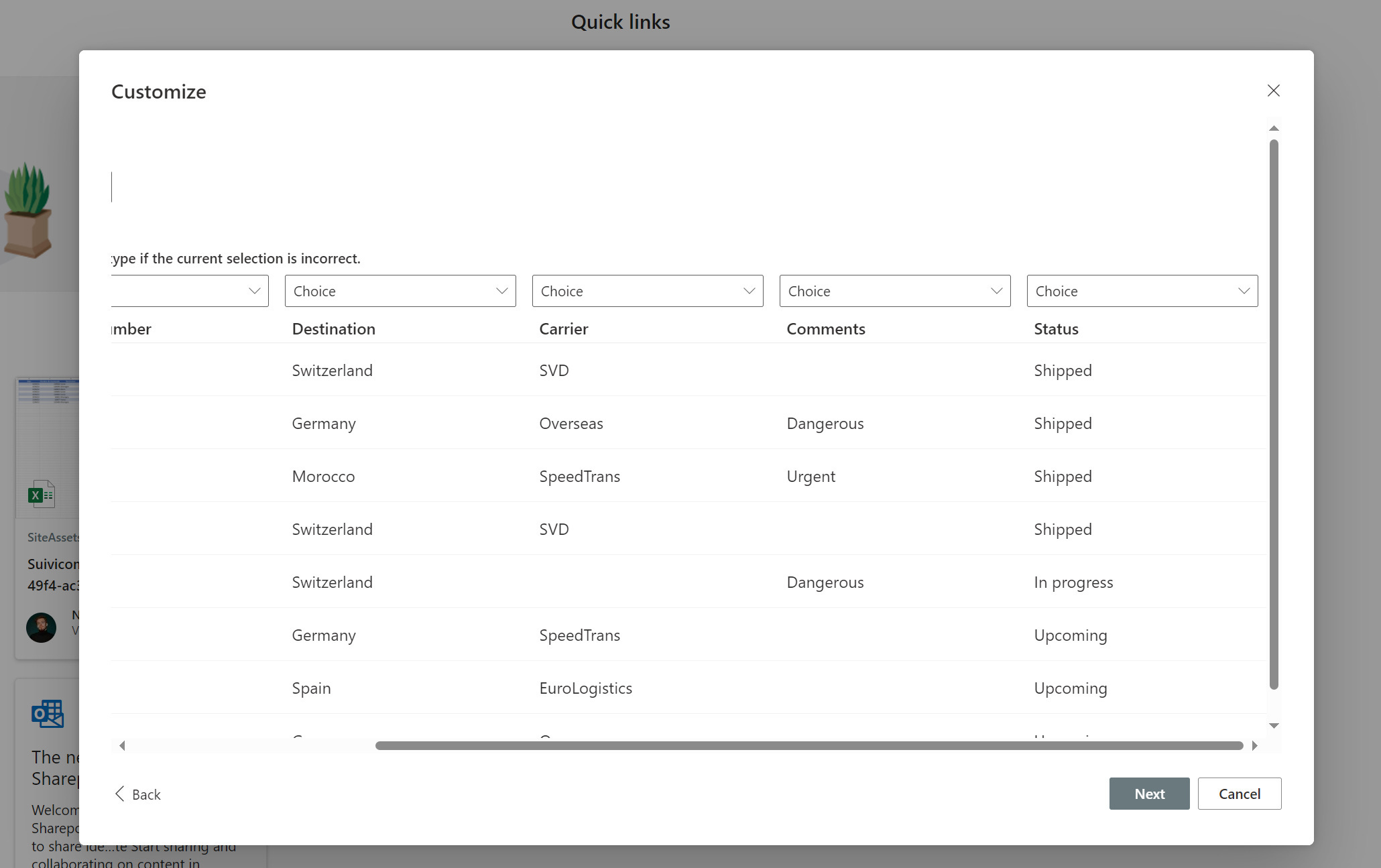
As for the other columns, we're going to cover a good practice you should remember when creating SharePoint lists.
To limit typing errors, we're going to choose the "Choices" category AS MUCH AS POSSIBLE.
This will force users to select from a number of choices and not write the information themselves.
Remember: in our original table, we had statuses that meant the same thing but were written differently:
Ok Shipped
DONE
Shipped
Completed
Technically, this means the same thing. But when you want to run analyses and statistics on your data, you're going to pull your hair out.
There has to be a unique way of saying that the order has been completed.
Incidentally, I also suggest you choose the "Choice" category for ... all the other remaining columns. You'll understand why a little later in the tutorial, trust me.
Here's how it should look:
We can click on Next and call our new list "Orders Follow-up" and leave "View in site navigation" ticked for easy retrieval.
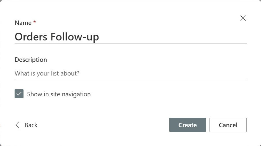
Click on "Create" to make the list available.
And that's it, after a few seconds our list is finally available, and we'll soon be able to bid farewell to our Excel file!
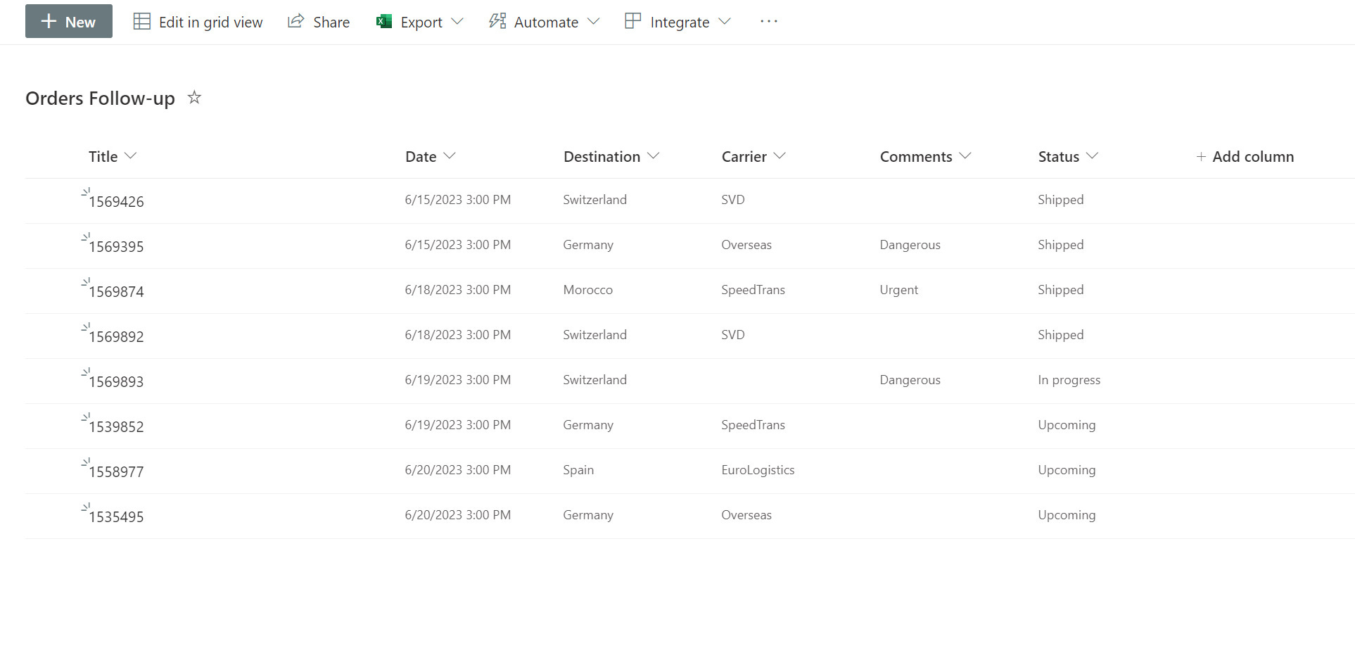
However, our work isn't finished yet, so follow me for the finishing touches.
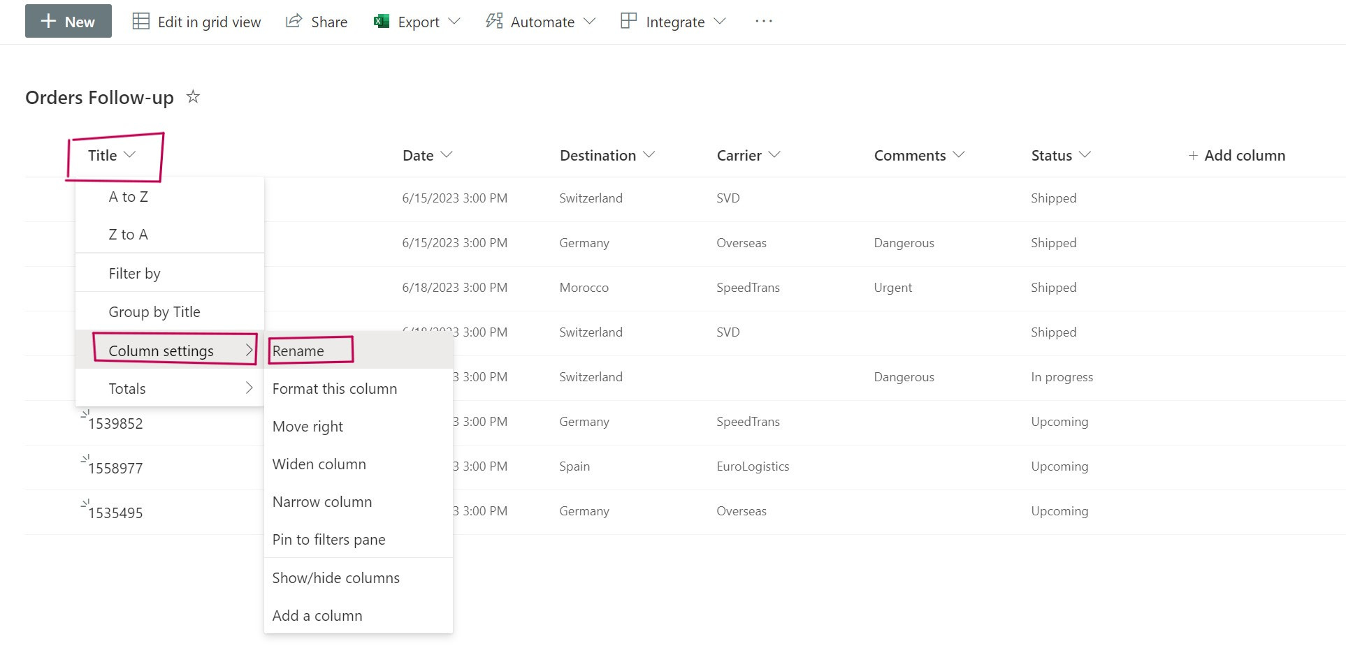
First, let's rename our "Title" column to "Order number" to make it more meaningful.
Click on the "Title" column, then "Column parameters" and "Rename".
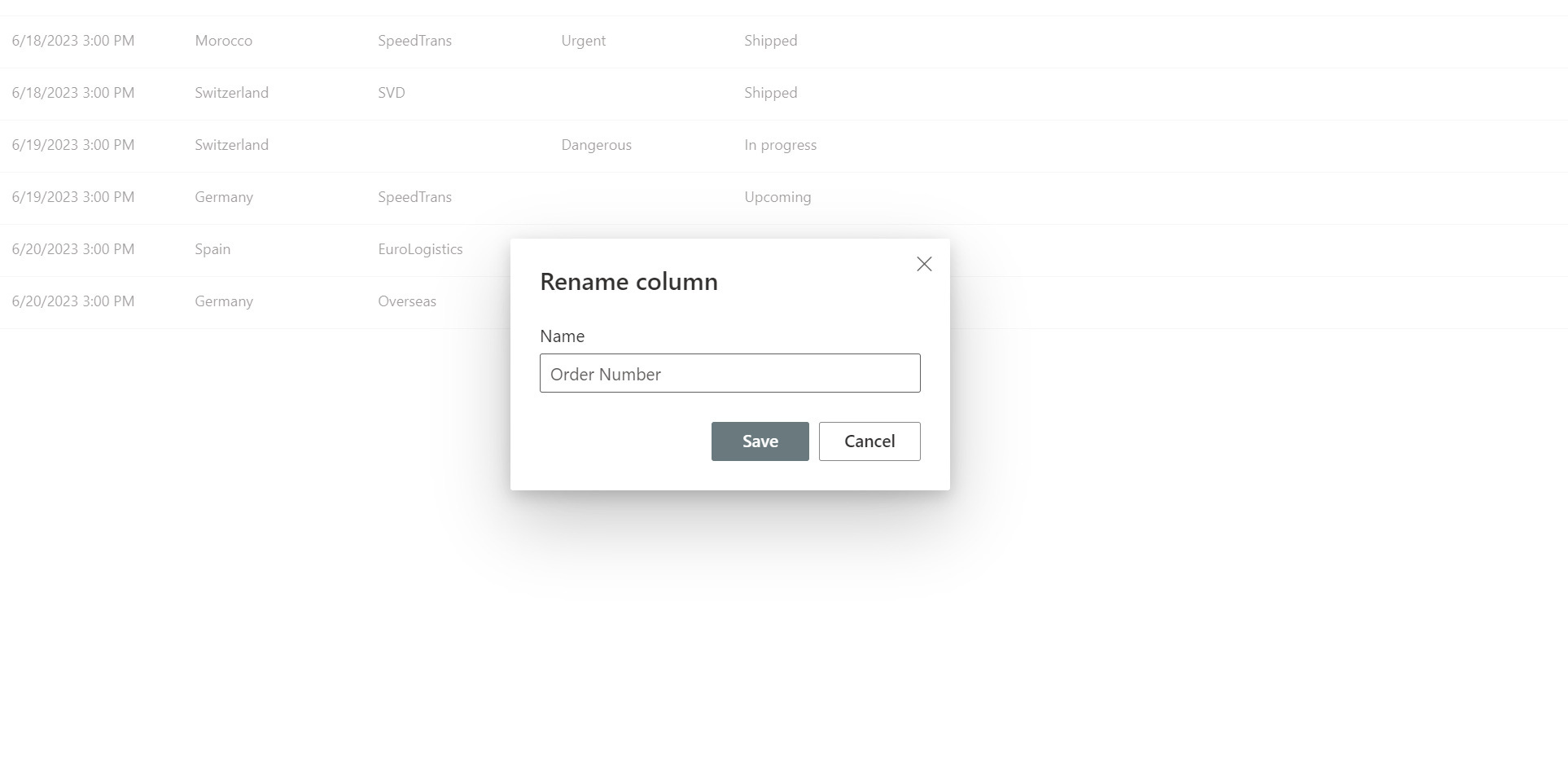
Rename to "Order number" and save.
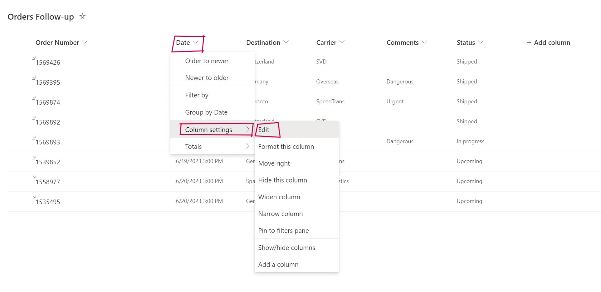
Now we're going to remove the time that was added after our date.
To do this, we'll click on the "Date" column, then "Column parameters" and "Modify".
In the window that opens on the right, we're going to uncheck "Include time" and take the opportunity to make the addition of information in this column compulsory, as follows:
Press Save at the bottom of the window and let's tackle the remaining columns, those to which we had assigned the "Choice" category.
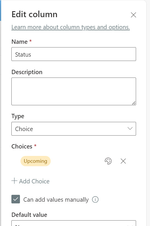
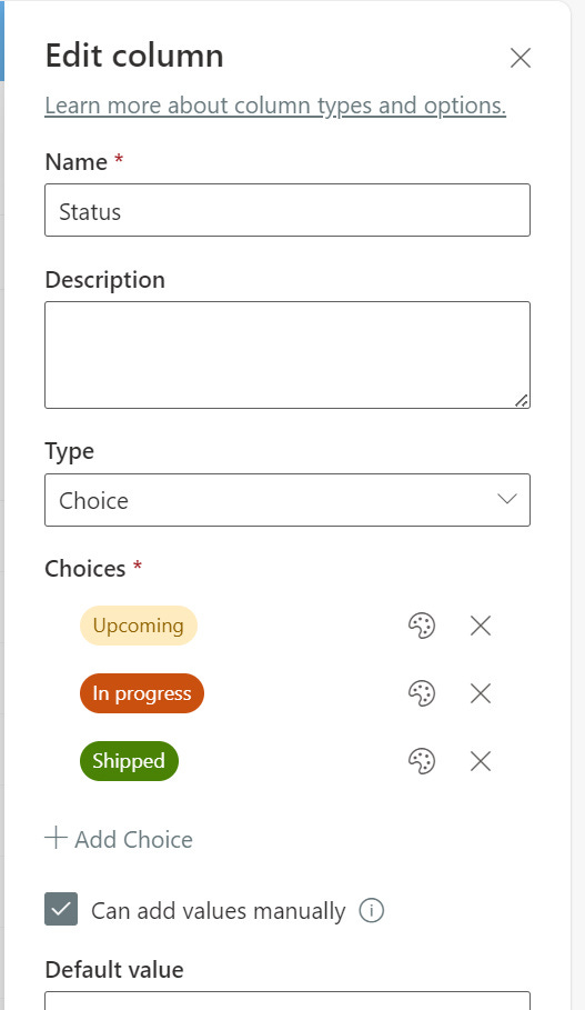
Click on the "Status" column, then "Column parameters" and "Modify".
The aim is to add the choices that users will have to select when adding or modifying an item.
Aside: An item is a record in a SharePoint list. For example, here are two items in our list :

We want to add the following choices:
Upcoming
In progress
Shipped
We'll simply click on "Add choice" and fill in Upcoming. On the palette to the right of the text, for example, we'll select the color yellow. Our choice should look like this:
We'll add the other two using the same procedure. In progress will be orange and Shipped will be green:
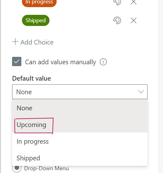
To make it easier for users to add a new order, we can assign a default value. Since the order will inevitably be Forthcoming, we can choose this in "Default value" :
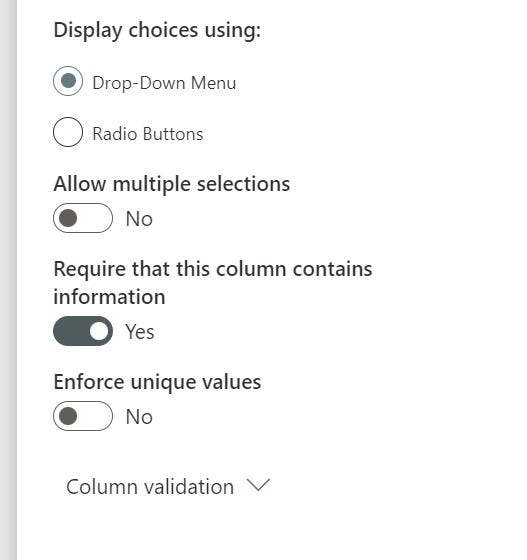
We will also make this field mandatory in the same way as the date:
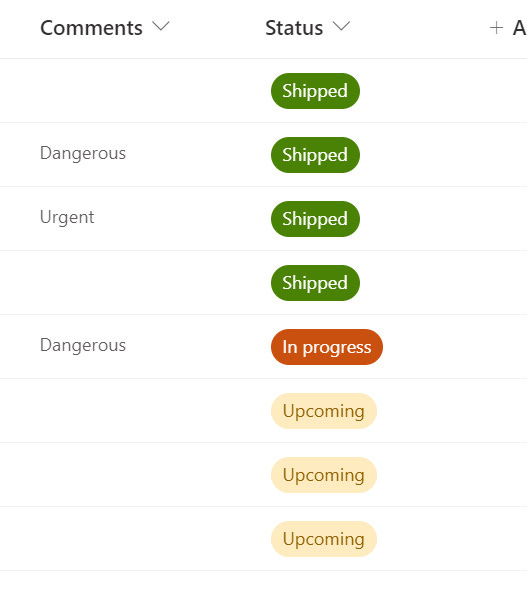
You can save and see that the info in the "Status" column now has a color corresponding to the one we've just assigned!
Let's do the same for the "Carrier" column, knowing that our carriers are :
SVD
Overseas
SpeedTrans
EuroLogistics
Your window should look like this:
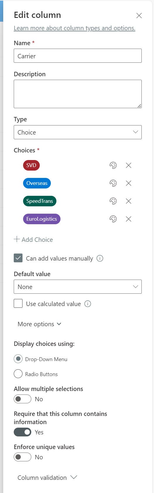
We don't select a default carrier, as it may change with each new order added to the list.
You've probably already noticed that we have a typo in one of our lines, as the carrier is missing. We've made the column mandatory, so SharePoint wants us to add the missing item.
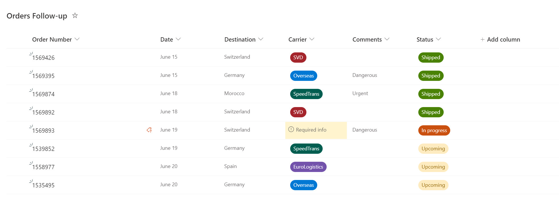
You can click on the offending line and then click on Modify above to fill in the missing carrier.
We can add the carrier "SVD" in the missing field and see that our list of choices appears correctly as below:
We can close this window and then go to the "Comment" column.
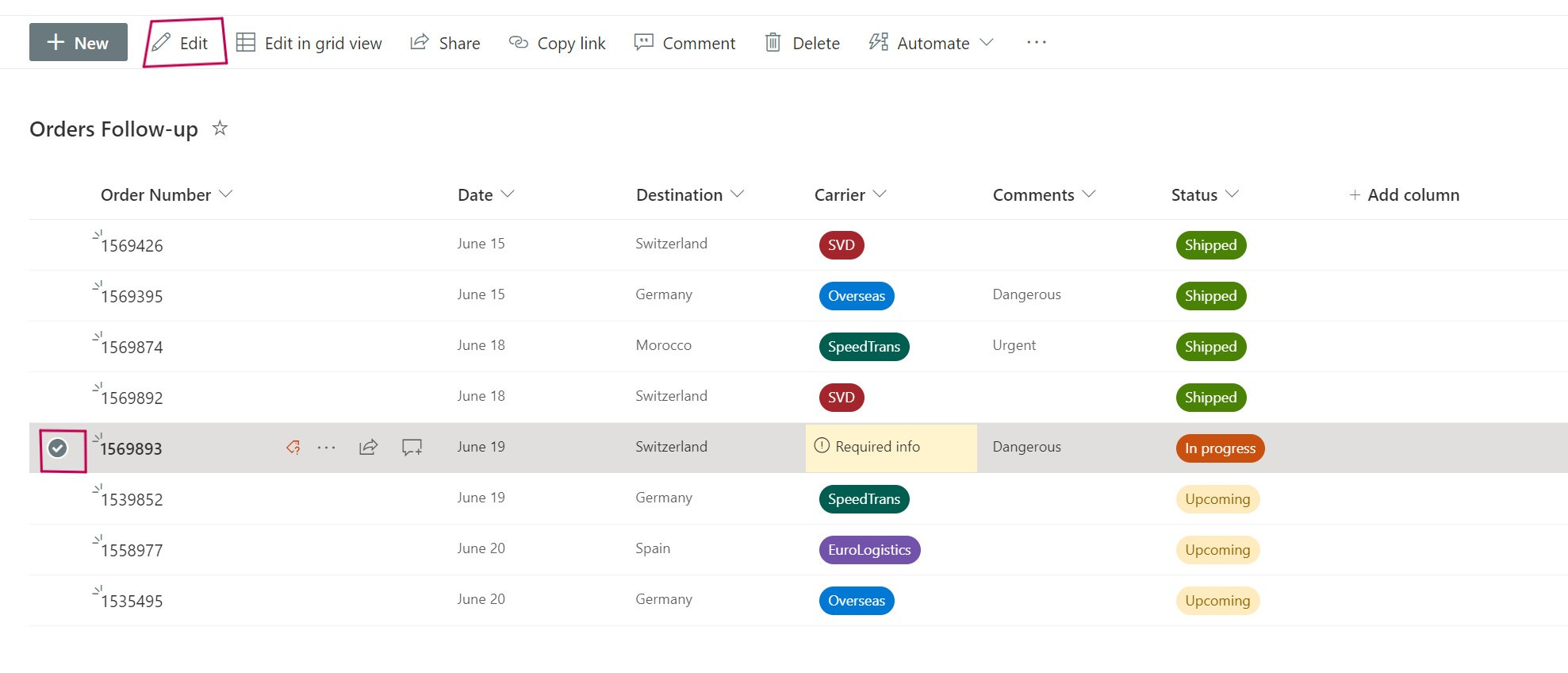
To begin with, let's add to the choices the comments we regularly find on commands:
Dangerous
Urgent
Fragile
We also know that the "Comment" column is optional, so we won't make it mandatory this time.
There's also a peculiarity: an order could be both "Fragile" AND "Urgent". So we're going to allow users to select more than one choice if they need to, by clicking on "Allow multiple selections". Your window should look like this:
After saving, let's go to the "Destination" column to add the names of the countries we trade with. One country corresponds to one choice.
"But imagine I have 50 destination countries, I'm not going to type them all in by hand!"
In fact, there's a little time-saving technique: we're going to use artificial intelligence to help us!
1- Go to : ChatGPT (openai.com)
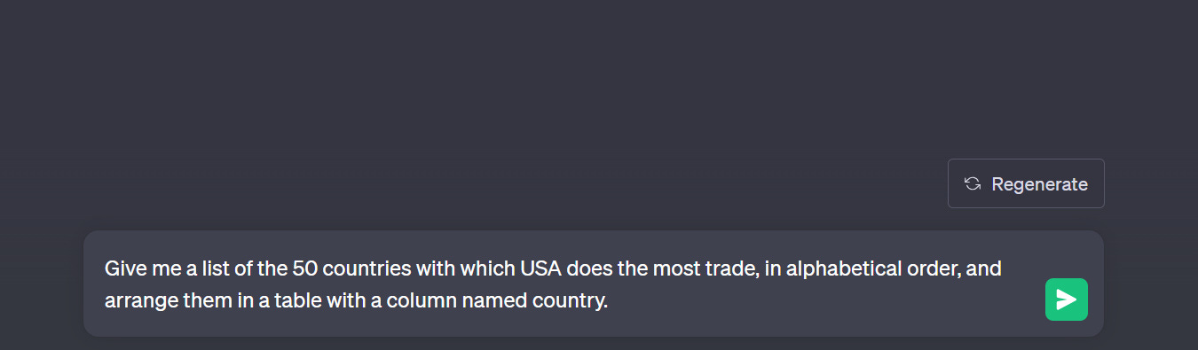
2- Create a new conversation and ask it the following:
"Give me a list of the 50 countries with which USA does the most trade in alphabetical order and arrange them in a table with a column named country"
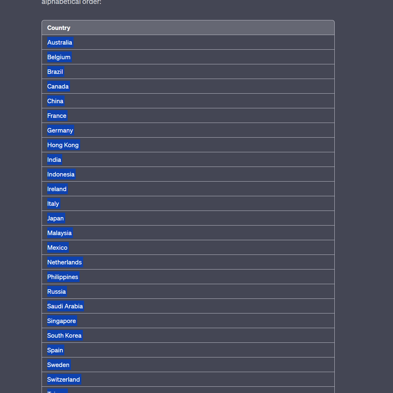
3- He should provide you with a fairly substantial list of countries. For some obscure reason, he hasn't sorted the last ones alphabetically, but that's not important (if you really want to fix it, you can ask him to correct or sort them yourself in Excel).
4- Select his table WITHOUT taking the title and right-click, copy :
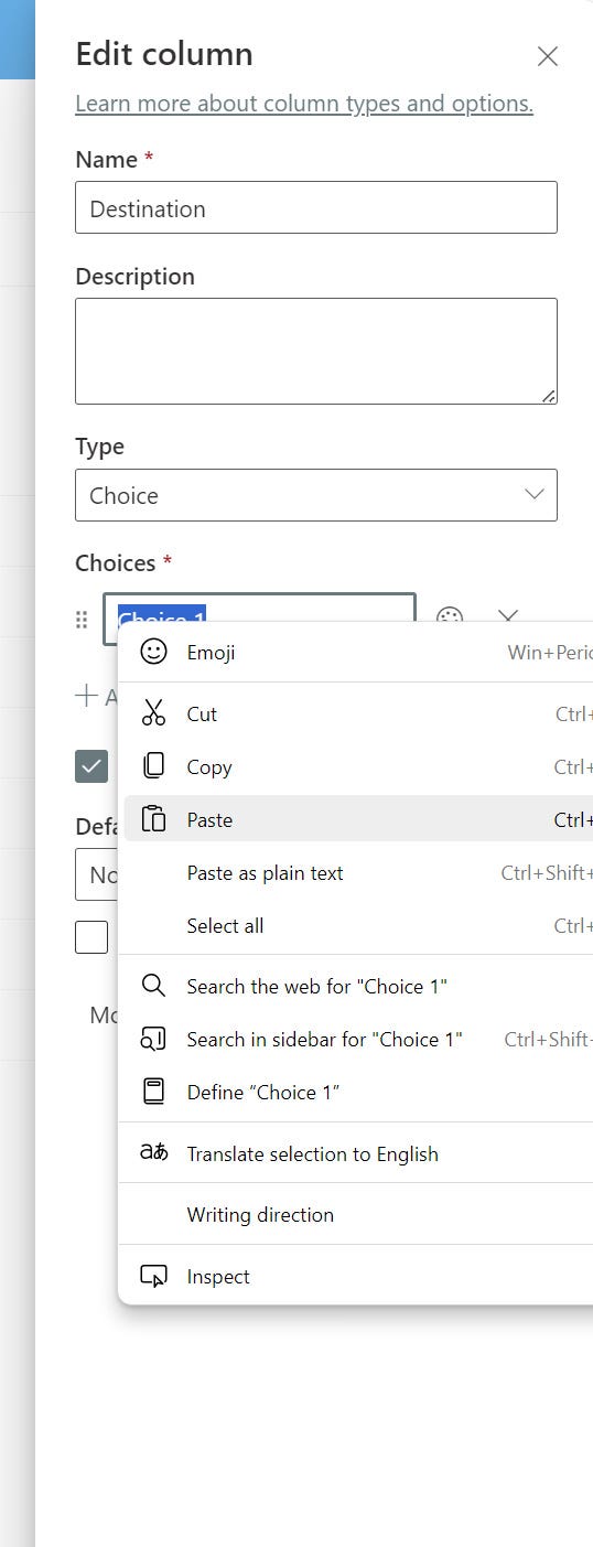
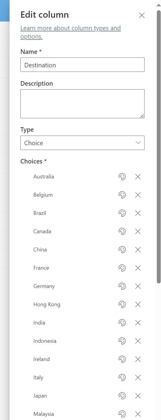
Then go back to your list, select "Add choice" and on "Choice 1", right-click and paste.
All your choices will be added automatically (pretty cool right?):
Don't forget to make this column mandatory before saving!
Well, we're nearing the end. And yet, there's still one essential thing to do: make the "Order number" column mandatory.
But we can't do it in the same way as the others. You can't access the column parameters by clicking on the column name this time!
Here's how it works.
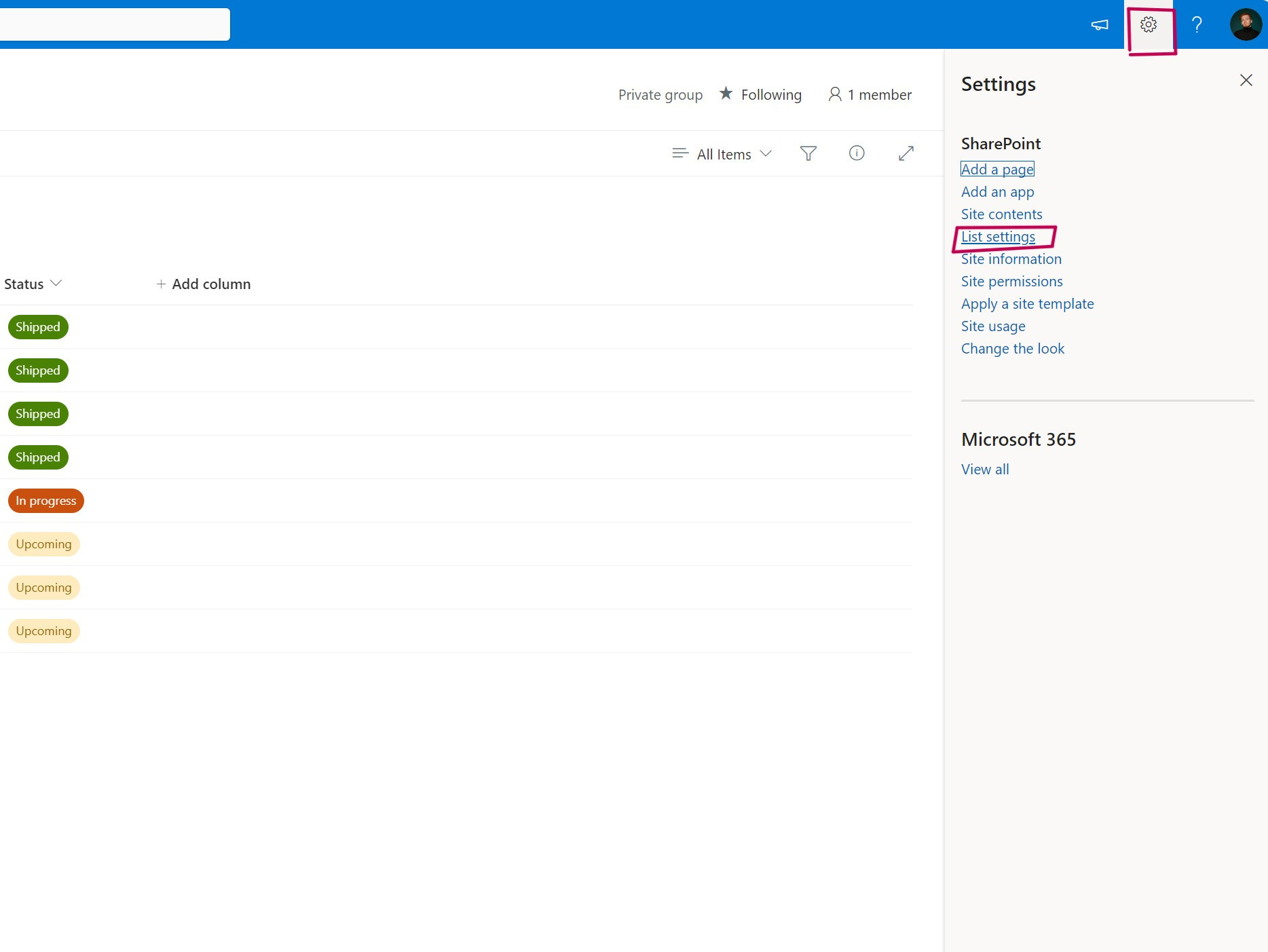
Go to the gearbox at the top of your list, then click on List settings:
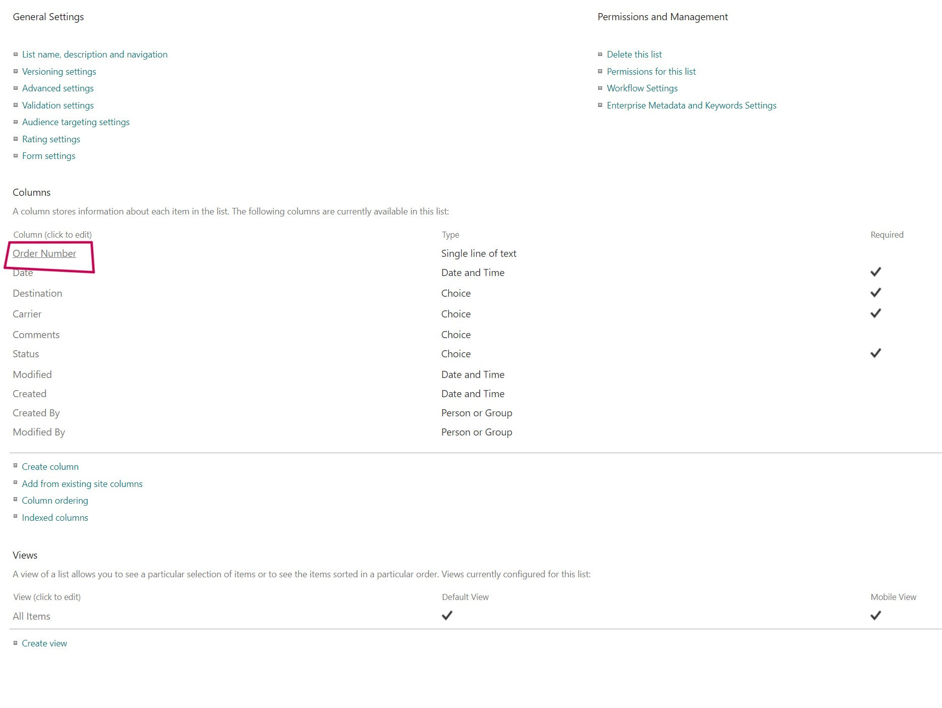
We will then go to the "Order number" column name below:
All we have to do is click "Yes" to the question "Require that this column contains information" and also “Yes” to enforce unique values in order to avoid having two similar order numbers:
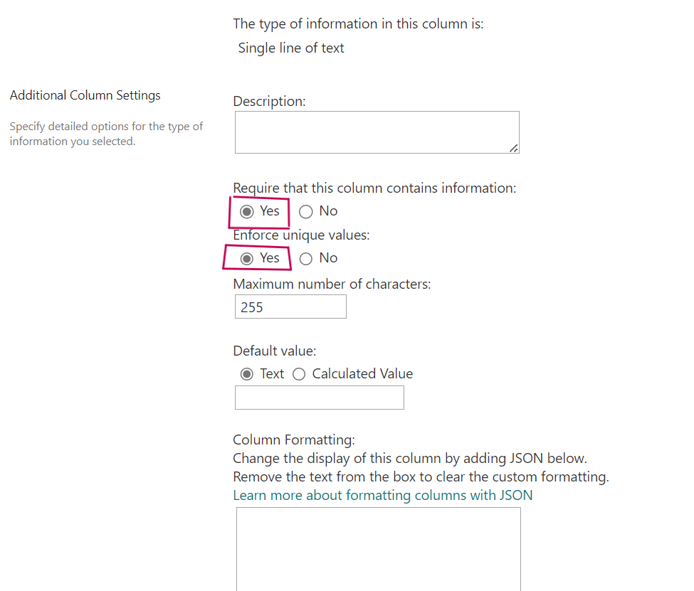
Click on Ok in the bottom right-hand corner of the screen to validate.
Congratulations, your list is now ready to use!
I hope you've enjoyed this first tutorial. Don't hesitate to subscribe to my newsletter to get access to new tutorials as soon as they're released!